Go ML - Vol 2

28th Apr 2021

Go Machine Learning Multivariate Linear Regression Mean Normalization

In the last article I introduced the command line utility I've been building in Go. In this article I'm going to get a bit more into the weeds with some machine learning concepts and how they are implemented in the tool. Nothing has really changed with the tool since the last article (I've a lot going on, get off my back, alright?!?!), but I'm going to hopefully give a bit more background on some of the cooler things the tool is capable of.

The TL;DR

In this article I'm going to be talking in detail about ML, so, unlike most of my articles, there isn't really a TL;DR...sorry, I guess. If you aren't interested, I suggest you skip this one!!

NOTE: I AM NEITHER AN EXPERT IN GO NOR ML, SO THIS MIGHT ALL BE GARBAGE

Multivariate Linear Regression

Multivariate liner regression can be a little confusing at first. Specifically the use of the word linear can be confusing, when in fact, multivariate "linear" models can be fit to...curves...CURVES, wat?!?! Yes, that's correct! When we dig into the maths a little bit, it becomes more obvious how the model I previously described for fitting a line can be used to fit a curve. However, we will talk more about that later. For now, lets write an expression that we can use as an example of multivariate linear regression.

Consider the following formula, y = x0.θ0 + x1.θ1 + x2.θ2, this should look fairly similar to our previous equation of the line y = m.x + c. In the new equation we have replaced c with x0.θ0, by convention we set x0 = 1 so c =~ θ0. Looking at the two equations, it more or less looks like we have taken two m.x terms and added them together along with the contant or offset term c. This is because that is exactly what we have done! The important part to not here is that each of our x terms are unique independent variables; x1 and x2. As it happens, this is the largest amount of independent terms that can be easily graphed.

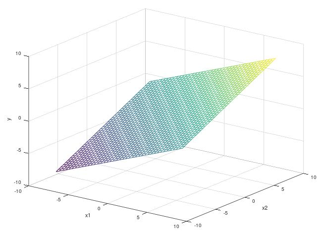
The above plot is what we call a surface plot. In the above example we have put x1 and x2 on the x and y axes respectively and our output y is on the z axis. Unlike our previous straight line examples, to try fit something to this shape, we need to figure out what values of θ minimize the error of two independent values. This sounds...tricky!

Before we figure out how we are going to solve this problem for multiple variables, lets revise how we do it with one. We wish to minimize the error of our predictions based on changing the value of θ. We can do this by using a process called gradient descent. For a single variable we can derive the update rule to tune the value of θ to be as follows: θ = θ - a/m.∑(y - ytrain) (y) So... now if we have θ1 and θ2... what do we do? Weirdly enough, we do the exact same thing!! It turns out that the derivation for the above equation works out to the same result regardless of how many parameters you have. The reason is actually pretty simple. Without going into the entire formal derivation, there is a step in the process where we compute the partial derivative of the initial equation for y. The cool thing about partial differentiation in this case is that while differentiating with respect to one of our parameters θn, the others all get treated as constants and so they end up disappearing in the derivation.

As I mentioned earlier, aside from multivariate linear regression being able to model multiple unique variables, it can also model curves. Amazingly, again, it works out of the box with no modifications to the process. This is pretty cool and feels like magic, so how does it "just work"? The confusion can lie in how we think about the linearity of the equation we are fitting to and the equation we are actually minimizing. The trick is that you need to think about what you are minimizing the equation in relation to. When you consider an equation like this y = θ0 + x.θ1 + x2.θ2, we know that this is a quadratic or "U-Shaped" curve. Importantly, this is not a line, and so how can linear regression minimize the error? The answer to this refers back to the partial derivative I mentioned earlier. When we are computing the derivative of our prediction function, we know the values of x. Tt is the values of θ that we don't know. In words, we are computing the partial derivative of the prediction with respect to the unknown parameters θ. So when we do the computation, the values of x and x2 become constants and disappear. So with respect to the parameters θ, the equation we are minimizing is always linear. Once we have computed constant values for θ, we can change our perspective on the equation again and hold them as constants and vary our values of x again to see our results.

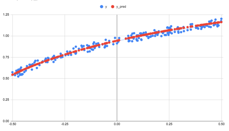
Below is the graphed output from the command line tool which is approximating the value of the natural logarithm function with some random noise applied to it. The fit was made using a non-linear function involving a square root term. As you can see, the error has been fairly accurately minimized.

Mean Normalization

So, what to you mean??... I'll get my coat. Terrible, terrible jokes aside, mean normalization is an interesting topic I want to spend some time diving into next. When I speak about mean normalisation, I am talking about a technique of feature scaling that can improve our learning algorithms in a few way.

To build some intuition as to why we would do this, lets consider a practical example. Imagine we want to predict house prices. To do this, we are going to look at two features which will become the two parameters of our model. These are, the size of the house in square meters and the number of bedrooms it has. Our formula will more or less be something like house price = θ1.number bedrooms + θ2.square meters. Lets now think about the scale of each of these quantities. House price is going to be in hundreds of thousands, the number of bedrooms is going to be in ones or maybe tens and the square meters might be in hundreds. When we train a learning algorithm to perform regression (predicting a continuous value, like a house price), we are really figuring out by what factor to multiply each of the parameters by to give the desired output. So lets consider our above example again; we are going start both of our θ values with a guess of lets say 1. If we want to get to the result that a house with 3 bedrooms and size 300 square meters should cost 300,000, we need to potentially end up weighting the size of the house by 100 and weighting the number of bedrooms by 1. This will give us a pretty close estimation of the actual result. However, the issues should be obvious here. It would take a massive change in the number of bedrooms to change the output of the model. So much so, that we might as well just ignore the number of bedrooms. Now, in real life often the number of bedrooms and size of a house are correlated but you could end up with a large house being built with a small amount of bedrooms. Maybe this house wont sell because no one wants to live in a 1000 square meter home with only two bed rooms. Our model will incorrectly predict it's price. This is a somewhat contrived example but the principle is still sound. Our model is unable to correctly assign feature importance purely because of the scales of the values rather than their actual importance.

Another subtle impact here is the amount of iterations it's going to take to get where we are going. As I said originally, we start at 1 and in our example we finish at 100. If we move by a very small step with each iteration, this gap is going to take a long time to bridge and we are wasting iterations just to get there. It would be way better if we could make our algorithm have to make fewer steps to get to the final answer.

Finally, there is a practical point here in the total size of the numbers we might have to deal with. If you want to fit a very complex set of high order features to a model; you could end up looking at features on the order of x6 or higher. Humans aren't very good at naturally grokking the scale of large numbers. However, trust me when I say if you start raising relatively small numbers to more than a power of 2 or 3, the results get very, very big. If you are limited to using the standard data types in a lot of commercial general purpose programming languages, you could overflow this. For example, in this command line tool, I use the float64 data type for most computations. It's max size is about 1.8*10308, that number is so large no human could ever comprehend any physical quantity it might relate to... and I managed to overflow it! All while messing with some code to take relatively small numbers and fit them to a model with high order features, who knew. The lesson is, my code is bad, and, make your physical numbers smaller and any programming language should be better able to deal with the outputs.

So we understand what the problem is, and what we should do about it. So, what DO we do about it? We mean normalize of course! The formula for this is as follows xnorm = (x - xavg)/(xmax - xmin). When we apply this to a set of inputs, it has the effect of scaling all the inputs relatively to between approximately [-1,1]. So that solves our large number problem. We also apply this formula uniquely to each set of inputs. This conveniently scales each input down to approximately the same scale. This then ensures that each features has equal chance to contribute to the final output.

You can find some not so pretty Go code here that automatically performs mean normalization on a matrix of inputs. The code might not be super slick, but there is some clever maths behind how to do this for a range of inputs in one go by using a vectorized implementation. Let's rearrange our formula to look like this xnorm = (1/r).x - k where r = xmax - xmin and k = xavg/r. 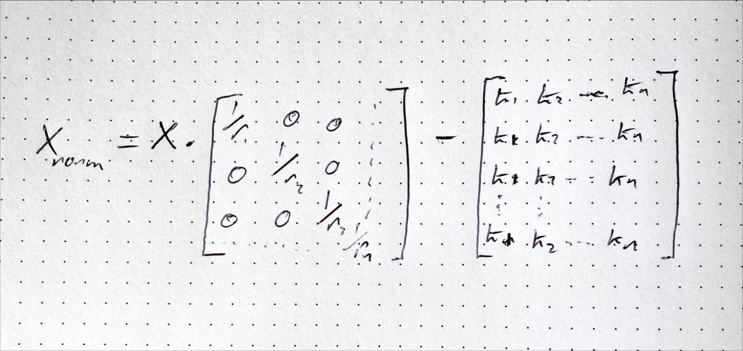We now have something that looks pretty much like the equation of a line. We can compute this generically for any matrix as follows. Xnorm = R.X - K (capitalization indicates a matrix). Importantly, the R matrix is a diagonal matrix in which each value is 1/r as pre computed for the column.

The above still requires that we compute the mean and the "range" of each set of inputs. However once we have these; we can compute the full set of scaled inputs in one line of linear algebra. That is kind of cool and also pretty computationally efficient, neat!

So, how's it Go-ing?

The more I am writing Go, the more I'm enjoying the patterns involved in using the language. So far, so good! However, one gap I have in my knowledge is how Go does memory management under the hood and how it handles passing around pointers. I have mostly been taking my queue from what libraries require to be passed in and making my code work around that. So I definitely need to pick up some knowledge there. I'm sure it's all obvious, however coming from high level languages where we just take that stuff for granted, I want to relearn it again and how it applies here in Go land.

One comment I have around working with Go for linear algebra is that the go-num library is a little hard to use. Don't get me wrong, the library certainly works and does do most of what I want. The issue is the syntax and some of the API surface. It's a little clumsy to use and some methods don't exactly work the way I would expect. Once you have your variables set up logically and you map out what gets passed to what, it makes sense and can be easy enough to follow. However, if you come from R, MatLab, Octave or even Python, the syntax feels messy and clunky. If I needed to test some linear algebra quickly, I'd probably default to Octave (it's free, I already have it and I happen to know it already 🤷‍♂️) to check that my maths is correct. I'm doubtful that I'd spin up some Go code to try quickly test out some linear algebra.

What's Next?

Honestly, I'm not sure! I have had a lot of other project on the...Go...recently (I don't know why I'm like this). So I haven't had much of a change to sit and write code or write words for that matter. I will probably look at adding logistic regression to the library next and don't you folks worry, I'll tell you alllllll about it. So until next time!

Keep on machine learning 😬
- Ian

If you enjoyed reading this article and would like to help funding future content, please consider supporting my work on Patreon.